6. Validations
This package also provides tools to validate interpolation methods, i.e., to estimate uncertainties due to interpolation. We here discuss the validation methods we propose, show some of the validation results, and introduce the procedure for users to test their interpolator or their grid data. The validation results are provided in validations/ directory of this package, together with all the codes to generate the results.
We propose and use two methods for validation. One is based on comparison among several interpolator; it is simple and gives a good measure of the error estimation due to interpolation. Another one is what we call “sieve-interpolation” results [1], which gives strict upper bounds on the error of interpolations.
| [1] | Or tell me another better name, if you have. |
6.1. Notation
We use the following notations to discuss our validations. This package compiles each row of the grid data to \(({\boldsymbol x}, y, \Delta^+, \Delta^-)\), where \(\boldsymbol x\in P\subset\mathbb R^D\) is a parameter set with \(D\) being the number of parameters, \(y\) is the central value for cross section \(\sigma({\boldsymbol x})\), and \(\Delta^\pm\) are the absolute values of positive and negative uncertainties.
We here assume that the grid is “rectilinear”; i.e., the parameter space \(P\) is a \(D\)-dimensional cube sliced along all the axes with possibly non-uniform grid spacing. In other words, the grid is defined by lists of numbers, \([c_{11}, c_{12}, \dots], \dots, [c_{D1}, c_{D2}, \dots]\), where each list corresponds to one parameter axis [2], and all the grid points \((c_{1i_1}, c_{2i_2}, \dots, c_{Di_D})\) are provided in the grid table. Thus we can address each grid point by \(D\)-integers, \(I:=(i_1, \dots, i_D)\), which we will mainly use in the following discussion.
Each patch of tessellation can also be addressed by \(D\)-integers. In a \(D\)-dimensional grid, a patch is formed by \(2^D\) grid points and we use the smallest index among the points to label a tessellation patch. For example, a patch \(S_{i,j}\) of a two-dimensional grid is the square surrounded by the points \((\boldsymbol x_{i,j}, \boldsymbol x_{i,j+1}, \boldsymbol x_{i+1, j}, \boldsymbol x_{i+1, j+1})\), or more explicitly,
An interpolator constructs an interpolating function \(f: P\to \mathbb{R}\) from a grid table. It is a continuous function (at least in this package) and satisfies \(f({\boldsymbol x}_I)=y_I\). he interpolators of this package also gives interpolations for values with uncertainties \(f^\pm\), which satisfy \(f^\pm({\boldsymbol x}_I)=y_I\pm\Delta^\pm\).
| [2] | This array is equivalent to the levels attribute of MultiIndex used to describe the grid index of data-frame for \(D\ge2\). |
To discuss the difference between two functions \(f_1\) and \(f_2\), we define variations and badnesses. The variation \(v\) is defined by the relative difference, while the badness \(b\) is the ratio of the difference to the ther uncertainty; i.e.,
Though they are not symmetric for \(f_1\) and \(f_2\), the differences are negligible for our discussion.
The badness is a good measure to discuss the interpolation uncertainty. For example, \(b=0.5\) means the interpolation uncertainty is the half of the uncertainty \(\sigma\) stored in the grid table, where we can estimate the total uncertainty by
Accordingly, we can safely ignore the difference between two interpolations if \(b<0.3\) (or \(\sigma_{\text{total}}<1.04\sigma\)), while we should consider including interpolation uncertainty if \(b>0.5\).
6.2. “Compare” method
This method estimates the interpolation error by comparing results from several interpolators.
For \(D=1\), we have several “kinds” of Scipy1dInterpolator, while for \(D=2\), we have “linear” and “spline” options for ScipyGridInterpolator.
The differences among the interpolators will give us a good estimation of the interpolation error.
This method does not suit for \(D\ge3\), but such tables are not yet included in this package.
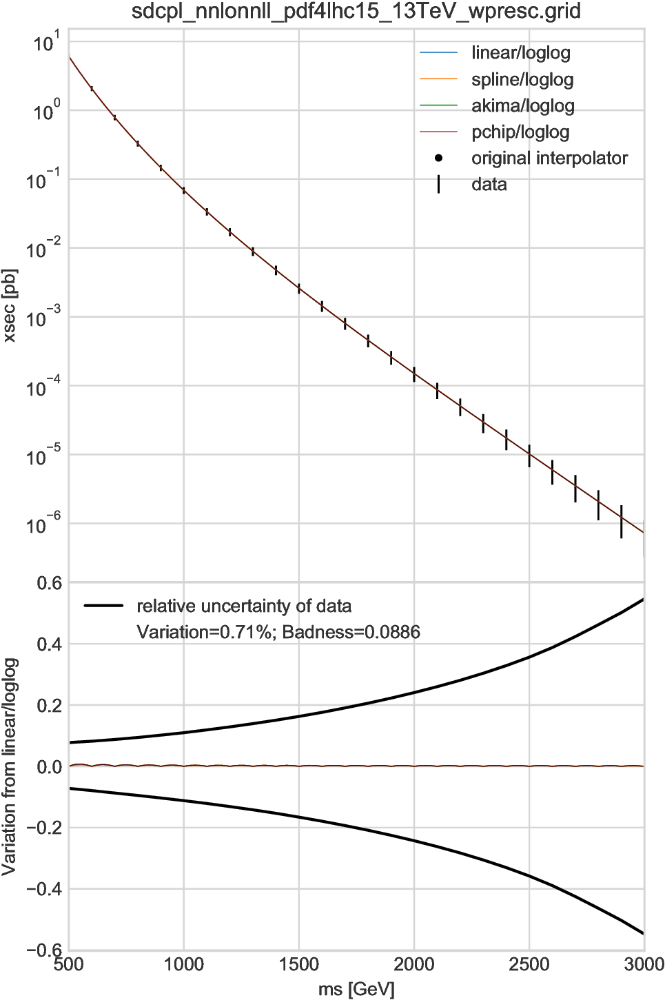
Fig. 6.1 For 13 TeV \(pp\to\tilde q\tilde q^*\) cross section.
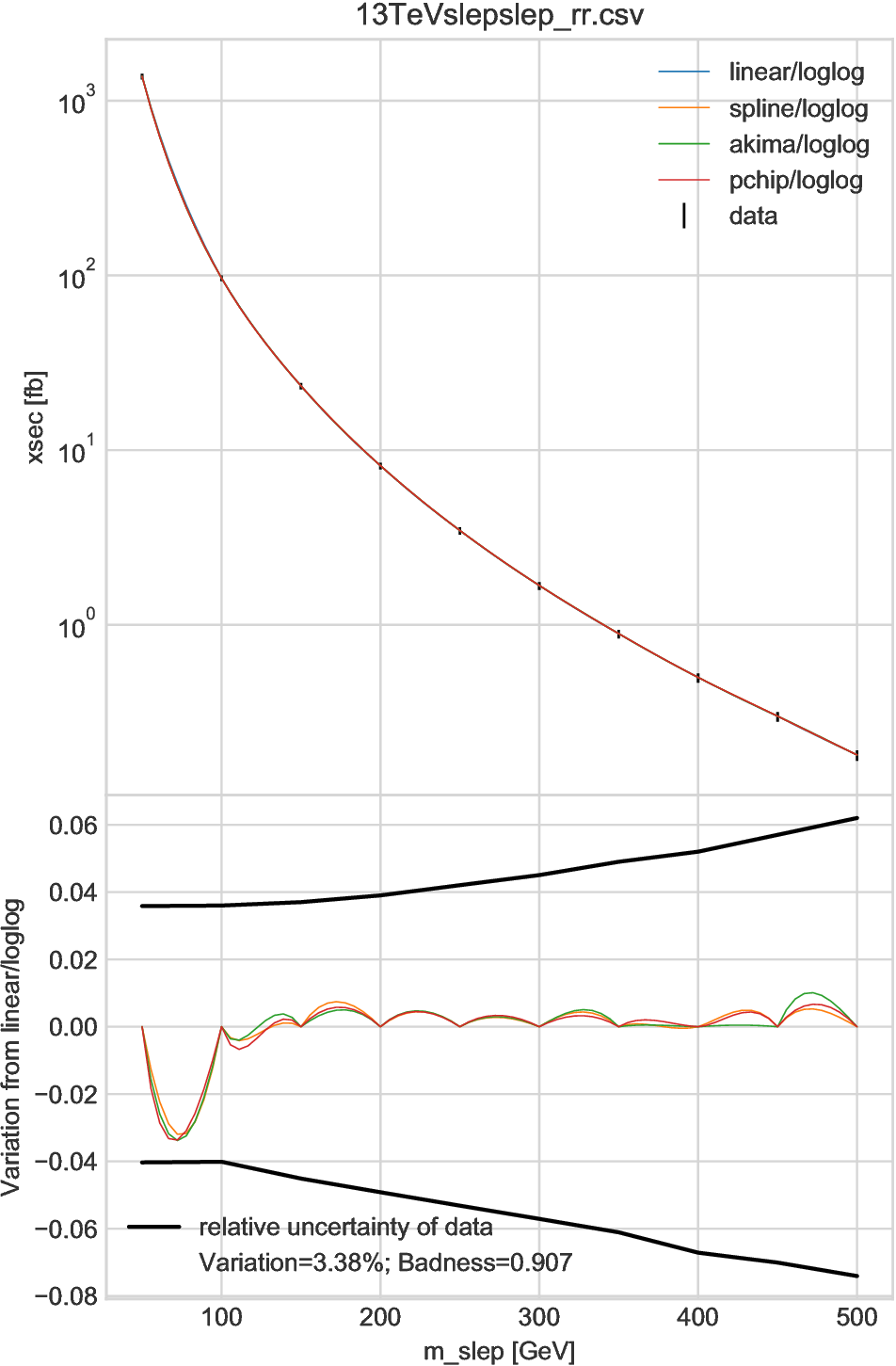
Fig. 6.2 For 13 TeV \(pp\to\tilde l_{\mathrm R}\tilde l^*_{\mathrm R}\) cross section.
Two examples of \(D=1\) are shown in Fig. 6.1 and Fig. 6.2, where the linear, cubic-spline, Akima [Aki70], and piecewise cubic Hermite interpolating polynomial (PCHIP) [FC80] interpolators based on log-log axes are compared to each other. In addition, for data tables provided by the NNLLfast collaboration (i.e., in Fig. 6.1), we compare our interpolators with their official interpolator; the results are shown by very tiny black dots, which may be seen as a black line overlapping the other results.
In the upper figures the interpolation results are plotted together with the original grid data shown by black vertical lines. All the results, crossing the central values by definition, are overlapped and undistinguishable. The lower plots show the relative differences between the linear and other interpolators. In Fig. 6.1 the badness is at most 8.9% and we regard those interpolators are equivalent. Meanwhile, in Fig. 6.2 the differences are visible. Especially, in the first interval, the linear interpolator gives a result considerably different from the other interpolators. which are all based on spline method and thus consistent, corresponding a badness of 0.91. Since we cannot tell which interpolator is giving the most accurate result, an interpolation uncertainty should be introduced for this interval, for example, by multiplying the other uncertainty by a factor \(\sqrt{1+0.91^2}\simeq 1.35\).
In general, the interpolation results are less accurate for the “surface” region of the parameter space \(P\), which corresponds to the first and last intervals in one-dimension case. For example, in the cubic-spline method, the functions of the first and last intervals are highly dependent on the boundary conditions. Thus users should be very careful if they apply interpolations to the surface regions in their analysis.
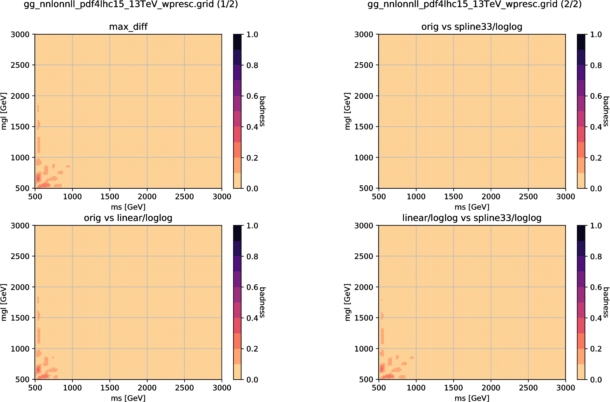
Fig. 6.3 A validation result of two-dimensional interpolators using the 13 TeV \(pp\to\tilde g\tilde g\) cross-section grid provided by NNLLfast collaboration. We here compare the linear and spline interpolators with the official NNLLfast interpolator (“orig”) and plot the badness, which is defined by the ratio of the difference to the other uncertainties. The upper-left plot shows the largest difference among the three comparisons, while the respective differences are shown in the other plots.
Fig. 6.3 shows a comparison result for two-dimensional case.
The linear and spline interpolators, together with the NNLLfast official interpolator, are compared in the gluino pair-production grid for the 13 TeV LHC.
The grid spacing is 100 GeV for both axes.
The spline interpolator (ScipyGridInterpolator with “spline” option) reproduces the official interpolator, while the linear interpolator has small deviations but the points with \(b>0.3\) is found only in the surface regions (“ms” or “mgl” less than 600 GeV).
Accordingly, these interpolators are equivalent for non-surface regions, while attention should always be paid for interpolating results of the surface regions.
Validation results for other grid tables are provided together with the package. For most of the grid tables the differences among the interpolators are negligible for non-surface regions, while significant differences are found in surface regions of some grid tables. While users should think of including uncertainties for interpolations in surface regions, one should keep in mind that this “compare” method is just a comparison and thus qualitative rather than quantitative. Thus we put further analyses out of scope of this package and left them to users. For details, see the files in validations/, where codes and instructions to generate the validation results by their own are provided.
6.3. “Sieve” method
This method gives a conservative estimation of the interpolation error by determining the value on a grid point from a “sieved” grid table, which is composed from the original grid table by removing every other line from all the parameter axes.
First, we formally introduce this method. Let us consider a \(D\)-dimensional parameter space \(P\) that is defined by the grids \([c_{11}, c_{12}, \dots], \dots, [c_{D1}, c_{D2}, \dots]\), as described above. Each grid point is given by
We can construct \(2^D\) sieved grid tables, labeled by \(P_{r_1r_2\cdots r_D}\) with \(r_n\) being 0 or 1, as
We can do interpolation over the sieved tables, but the resulting functions \(f_{r_1r_2\cdots r_D}\) should give much worse results than the original interpolation \(f\).
Let us consider a grid point \({\boldsymbol x}_{3,4,5}\), where we assume \(D=3\) for simplicity. The point is included only in \(P_{101}\), so \(f_{101}({\boldsymbol x}_{3,4,5})\) gives the true value \(y_{3,4,5}\), so does \(f\). Meanwhile, the other interpolations \(f_{ijk}\) do not give the correct value. In particular, the value is least accurate in \(f_{010}\) because all the neighboring points are not included in \(f_{010}\); the point \({\boldsymbol x}_{3,4,5}\) locates the central region of a patch. Therefore, the difference from the true value, \(\delta_{3,4,5}:=f_{010}({\boldsymbol x}_{3,4,5}) - y_{3,4,5}\), gives a good estimation of the interpolation error of \(f_{010}\) for the region close to \({\boldsymbol x}_{3,4,5}\). We use this difference and resulting variation and badnesses as the error estimation of the original interpolation \(f\) around \({\boldsymbol x}_{3,4,5}\).
In summary, the “sieve” method gives a very conservative estimation of the interpolation error around \({\boldsymbol x}_{i_1,\dots,i_D}\) for an interpolation \(f\) by
where \(\bar r_n:=(i_n+1)\bmod2\).
Note not only that this method does not give an estimation for the surface points, but also that, for spline-based interpolators, the estimation given by this method becomes extremely conservative for the next-to-surface and next-to-next-to-surface points because they locate at the center of a surface patch in the sieved grid table. Therefore, for spline-based interpolation, it will be ideal to prepare grid points with margins of two or three grid points beyond the region of interest.
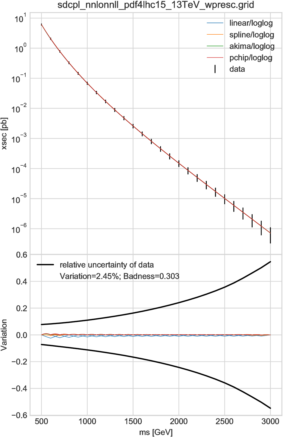
Fig. 6.4 For 13 TeV \(pp\to\tilde q\tilde q^*\) cross section.
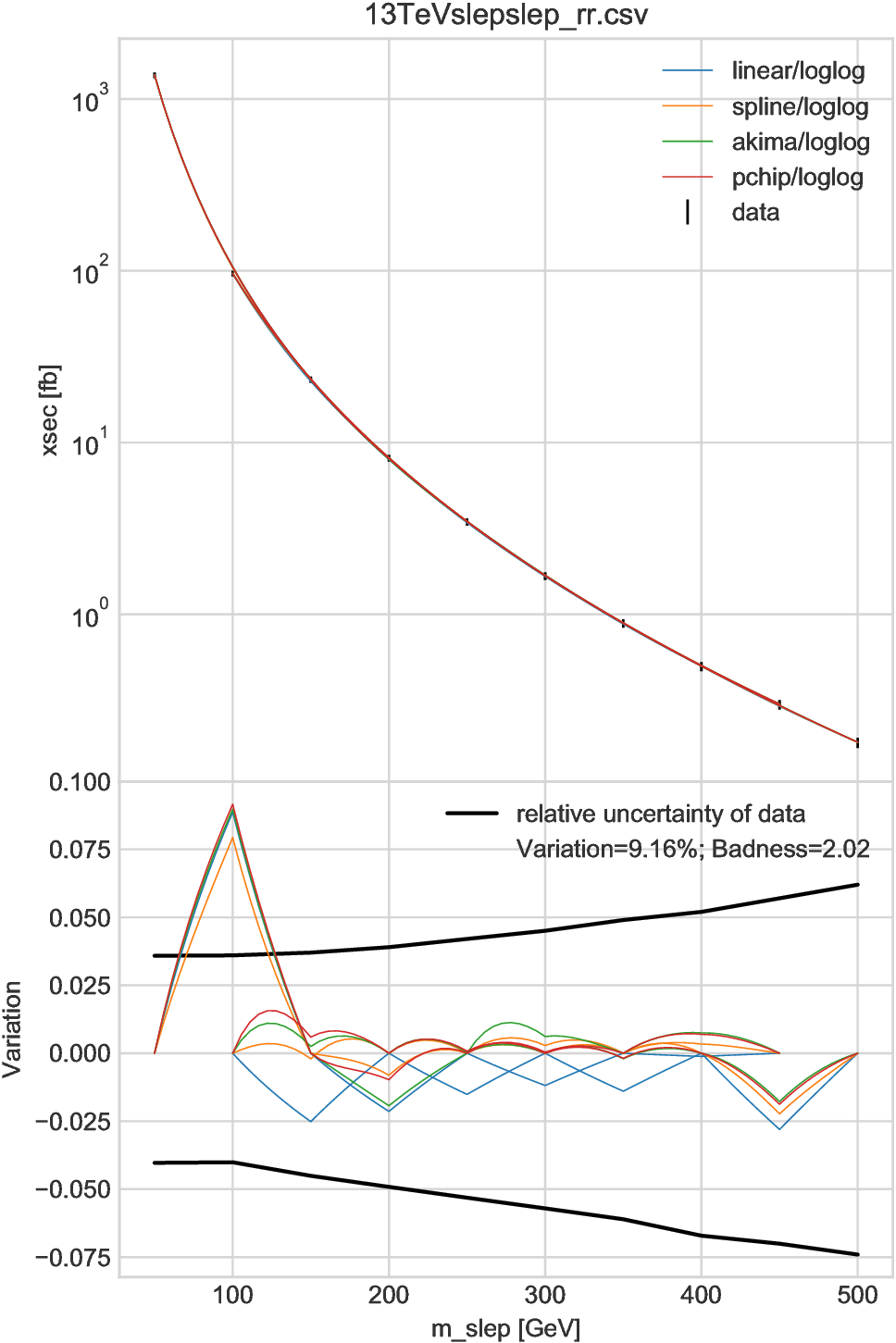
Fig. 6.5 For 13 TeV \(pp\to\tilde l_{\mathrm R}\tilde l^*_{\mathrm R}\) cross section.
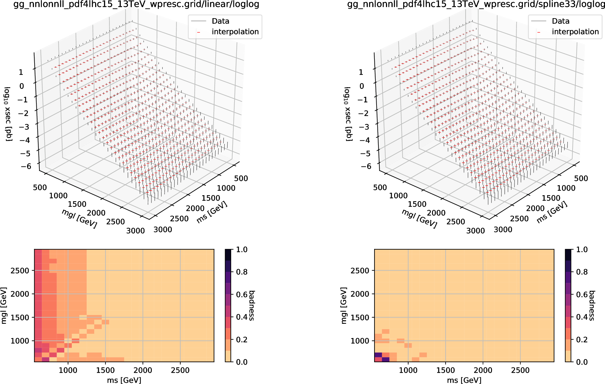
Fig. 6.6 A validation result of two-dimensional interpolators using the 13 TeV \(pp\to\tilde g\tilde g\) cross-section grid provided by NNLLfast collaboration. The left (right) figure is for the linear (cubic-spline) interpolator. In the upper plots the vertical intervals show the uncertainty range of true values and the horizontal ticks show the sieved interpolation results. The lower plots show the badnesses around each of the grid points.
Sample results are shown in Fig. 6.4, Fig. 6.5, and Fig. 6.6, which are for the same grid tables as in the previous section. In the first figure, \(D=1\) and thus two lines are shown for each interpolator. Those eight lines are overlapped and barely distinguishable; in the lower plot one may see two lines for the linear interpolator, which have a zig-zag form because each interpolator gives the true value at every other points. Since the maximal badness is 0.30, the interpolation error is negligible for this case.
A worse result is shown in Fig. 6.5, which indicates that we could not trust the interpolation for \(m_{\text{slep}}\lesssim125\,\text{GeV}\) if the grid spacing were doubled (100 GeV). Practically, one will avoid using the interpolation, consider to insert additional grid points, or include uncertainty due to interpolation based on the results of the “compare” method for this region. Conversely, we can safely ignore the interpolation error for \(m_{\text{slep}}\gtrsim125\,\text{GeV}\), which agrees with the “compare” method.
Fig. 6.6 is an example with \(D=2\); the left (right) figure is a validation for the linear (cubic-spline) interpolator. The upper plots include the sieved interpolation results \(f_{\bar r_1\bar r_2}({\boldsymbol x}_{i_1, i_2})\) as the horizontal ticks and the uncertainty range of true values as the vertical lines; by construction, the surface points lacks the sieved interpolation results. The lower figures show the badness for each grid point. Generally, the spline interpolator gives better results, and this is the reason we use the spline interpolato in get sub-command. Here, however, one should be careful of the surface region, where the interpolation result is affected by boundary conditions; in fact, the spline interpolator gives much worse results than the linear interpolator at the corner.
Validation results for other grid tables are provided together with the package. In general, as far as avoiding the surface region and the region next to them, the spline interpolator gives very accurate results and users do not have to care of the interpolation error. Meanwhile, the spline interpolation is less trustable for the first and second intervals, where one should consider introducing the interpolation uncertainty. For details, see the files in validations/, where codes and instructions to generate the validation results by their own are provided.
| [Aki70] | H. Akima. A New Method of Interpolation and Smooth Curve Fitting Based on Local Procedures. Journal of the ACM 17 (1970) 589–602. |
| [FC80] | F. N. Fritsch and R. E. Carlson. Monotone piecewise cubic interpolation. SIAM Journal on Numerical Analysis 17 (1980) 238–246. |